Earned Value Management Explained: EV vs PV, ETS Formulas, and Practical Application

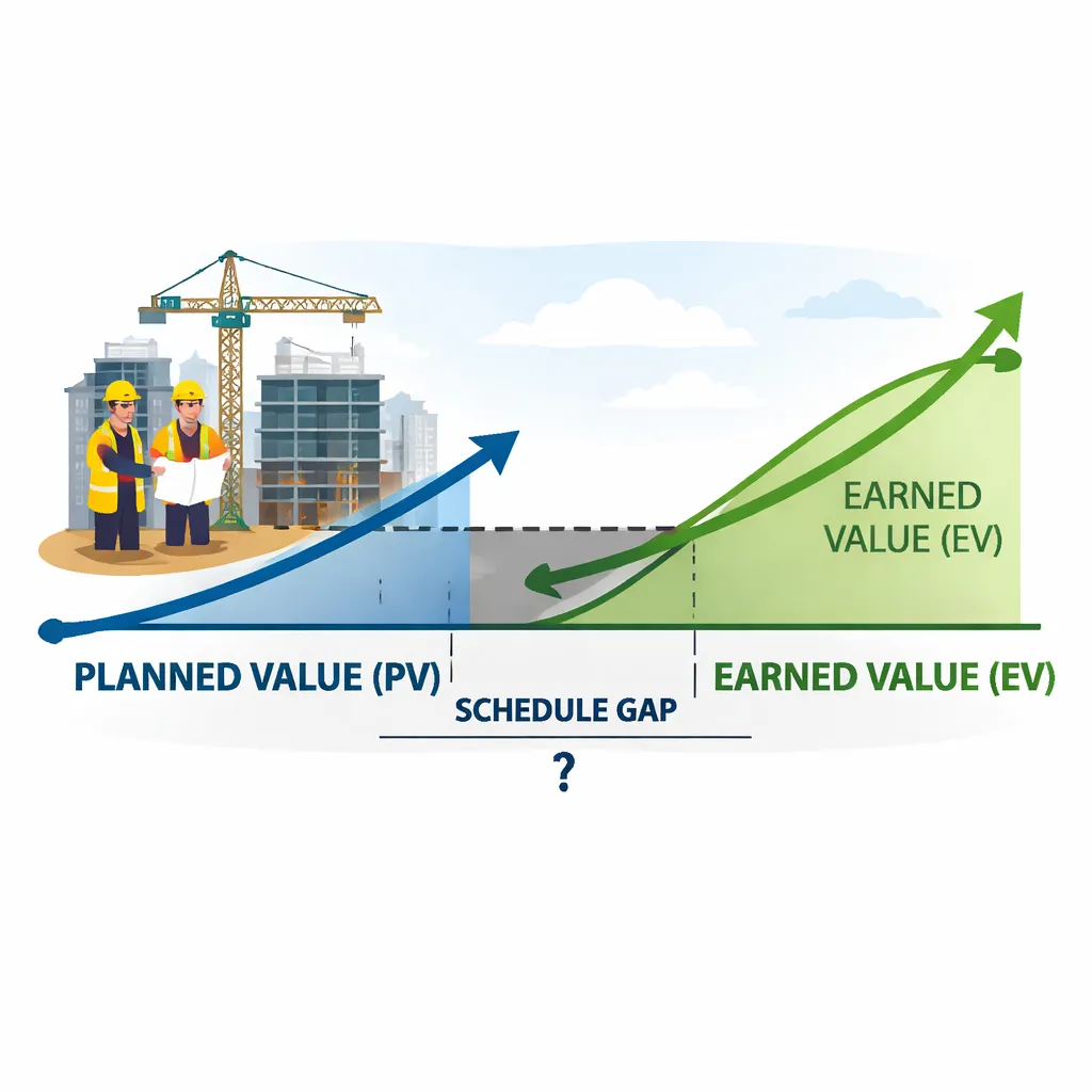
In the high-stakes environment of construction, simply tracking expenses against a budget is insufficient for understanding true project health. A project can be under budget but critically behind schedule, a reality that traditional accounting methods often obscure. This is where Earned Value Management (EVM) provides an indispensable framework. EVM integrates project scope, schedule, and cost into a unified system, offering a clear, objective measure of performance. For engineers and project managers, mastering EVM is not just about reporting; it's about gaining the foresight needed to steer complex projects toward successful completion. Accurate forecasting, a core output of EVM, is critical for managing stakeholder expectations, mitigating risks, and making proactive decisions before minor deviations become irreversible problems.

Understanding EV and PV in Earned Value Management

At the heart of EVM are two fundamental metrics: Planned Value (PV) and Earned Value (EV). While they may sound similar, they represent different sides of the performance coin—where you planned to be versus where you actually are.

What is Planned Value (PV)?

Planned Value (PV) represents the authorized budget assigned to the work scheduled to be completed by a specific date. It is the time-phased baseline against which project performance is measured. In simpler terms, PV answers the question: "What is the value of the work we planned to have done by now?"

• Calculation: PV is determined at the outset of the project during the planning phase. It is calculated as: PV = Planned % Complete × Budget at Completion (BAC)
• Function: PV serves as the performance measurement baseline (PMB). It sets the expectation for progress over time. If a project has a total budget (BAC) of $1,200,000 and is planned to take 12 months, the PV at the end of month 6 would ideally be $600,000, assuming a linear work distribution.

What is Earned Value (EV)?

Earned Value (EV) is the value of the work actually completed to date, measured in terms of the approved budget. It quantifies the progress in monetary terms. EV answers the question: "What is the value of the work we have actually finished?"

• Calculation: EV is measured by assessing the physical progress of the work and multiplying it by the budgeted cost for that work. The formula is: EV = Actual % Complete × Budget at Completion (BAC)
• Function: EV provides a realistic measure of accomplishment. Using the previous example, if at the end of month 6 only 40% of the total project scope is complete, the EV would be 0.40 × $1,200,000 = $480,000.

Key Differences Between EV and PV

The core difference lies in their perspective. PV is a forward-looking metric based on the project plan, while EV is a backward-looking metric based on actual accomplishment. Comparing the two provides an immediate and powerful indicator of schedule performance.

• PV is time-based: It reflects the value of work that should have been done according to the schedule.
• EV is progress-based: It reflects the value of work that has been done, irrespective of the time taken or cost incurred.

When EV is less than PV, the project is behind schedule. When EV is greater than PV, it is ahead of schedule. This simple comparison is the foundation of EVM's schedule analysis.

Performance Analysis Using EV and PV

By combining EV and PV with a third metric, Actual Cost (AC)—the total cost actually incurred to complete the work—we can perform a comprehensive analysis of both schedule and cost performance.

Schedule Performance

Schedule performance is measured using Schedule Variance (SV) and the Schedule Performance Index (SPI).

• Schedule Variance (SV): This metric shows how far ahead or behind schedule the project is in monetary terms. SV = EV - PV. A negative SV indicates the project is behind schedule. In our example, SV = $480,000 (EV) - $600,000 (PV) = -$120,000. This means the project is $120,000 worth of work behind its plan.
• Schedule Performance Index (SPI): This is a ratio that measures schedule efficiency. SPI = EV / PV. An SPI less than 1.0 indicates that the project is progressing at a slower rate than planned. In our example, SPI = $480,000 / $600,000 = 0.8. This means the project is progressing at only 80% of the planned rate.

Cost Performance

Cost performance is measured using Cost Variance (CV) and the Cost Performance Index (CPI).

• Cost Variance (CV): This metric shows whether the project is over or under budget for the work completed. CV = EV - AC. A negative CV indicates a cost overrun. If the Actual Cost to achieve the 40% completion was $500,000, then CV = $480,000 (EV) - $500,000 (AC) = -$20,000.
• Cost Performance Index (CPI): This ratio measures cost efficiency. CPI = EV / AC. A CPI less than 1.0 indicates that the project is getting less value than planned for every dollar spent. In this case, CPI = $480,000 / $500,000 = 0.96. The project is earning only 96 cents of value for every dollar spent.

Interpretation of Results: A Real-World Example

Consider a foundation-laying phase for a commercial building. The plan (PV) was to complete all excavation and rebar installation by week 4, valued at $200,000. However, due to unexpected soil conditions, only the excavation is complete, which was budgeted for $120,000 (EV). The actual cost (AC) incurred to do this was $150,000 due to equipment overtime.

• SV = $120,000 - $200,000 = -$80,000 (Behind Schedule)
• SPI = $120,000 / $200,000 = 0.6 (Highly inefficient with time)
• CV = $120,000 - $150,000 = -$30,000 (Over Budget)
• CPI = $120,000 / $150,000 = 0.8 (Highly inefficient with cost)

The data clearly shows the project is in trouble on both fronts. This allows the project manager to investigate the root causes—was the initial soil survey inadequate? Is the equipment inefficient?—and implement corrective actions immediately.

ETS (Estimated Time to Schedule) Formulas: Forecasting the Finish Line

Knowing you are behind schedule is one thing; knowing when you will actually finish is another. This is where Estimated Time to Schedule (ETS) formulas come into play. ETS, also known as Independent Estimate at Completion for Time (IEACt), forecasts the project's completion date based on current performance.

Why Do Multiple ETS Formulas Exist?

There is no single, universally accepted ETS formula because each one is based on a different assumption about future project performance. The choice of formula depends on the project manager's assessment of whether the current performance trends will continue, improve, or worsen. This analytical judgment is crucial for generating a realistic forecast. Advanced project scheduling and earned value management solutions often allow for the selection and customization of these formulas to fit specific project contexts.

Common Time Forecasting Approaches

Most ETS formulas use the Schedule Performance Index (SPI) as a key input, reflecting the efficiency of time utilization. Here are some of the most common approaches:

1. ETS = Planned Duration / SPI

This is the most widely used and straightforward formula. It assumes that the schedule performance efficiency (or inefficiency) observed to date will continue for the remainder of the project.

• Assumption: The factors causing the current SPI value (e.g., crew productivity, site access issues) will persist.
• Application: Best suited for projects where the current performance is believed to be representative of future performance. For our 12-month project with an SPI of 0.8, the ETS would be 12 months / 0.8 = 15 months. This forecasts a 3-month delay.

2. ETS = AT + (PD - ED)

This formula is more optimistic. It calculates the remaining duration based on the original plan, effectively assuming future work will be completed at the planned rate (i.e., with an SPI of 1.0).

• Assumption: The past schedule variance was due to a one-time event that has been resolved, and the project will get back on track.
• Application: Use with caution. This is only appropriate if a clear, actionable recovery plan is in place and its success is highly probable. (AT = Actual Time, PD = Planned Duration, ED = Earned Duration, where ED = AT x SPI).

3. ETS = AT + (PD - ED) / PF

This is a more flexible and sophisticated formula that introduces a Performance Factor (PF). The PF can be adjusted based on the project manager's judgment.

• Assumption: Future performance can be predicted more accurately by a specific factor. The PF could be the current SPI, the cumulative CPI, a combination (SPI x CPI), or another manually derived index.
• Application: Useful for complex projects where multiple factors influence schedule performance. For example, if both cost and schedule issues are systemic, using PF = SPI x CPI might provide a more conservative and realistic forecast.

Limitations of Each Formula

ETS formulas are powerful but not infallible. Their primary limitation is that they are mathematical extrapolations. They do not inherently understand the project's critical path, resource constraints, or external risks. An SPI might be healthy (e.g., 0.98), but if the minor delays are all on the critical path, the project's end date will still slip. Therefore, ETS should always be used in conjunction with Critical Path Method (CPM) analysis.

Which Method Is Better in Practice? A Guide for Engineers

Choosing the right forecasting method requires a blend of quantitative analysis and professional judgment.

Comparison of Formulas: Accuracy vs. Simplicity

The `ETS = PD / SPI` formula offers the best balance of simplicity and realism for most scenarios. It is easy to calculate, simple to explain to stakeholders, and grounded in actual performance data. While more complex formulas using a Performance Factor can offer more nuance, their added complexity can sometimes obscure the underlying assumptions, making them harder to validate and defend.

Project Type Considerations

• Repetitive Projects: For projects with linear and repetitive tasks, such as highway construction or pipeline installation, the `PD / SPI` method is often very reliable. Past performance is a strong indicator of future performance in these environments.
• Complex & Unique Projects: For one-of-a-kind projects like constructing a unique architectural structure or a first-of-its-kind industrial plant, past performance may be less indicative of future challenges. In these cases, a more analytical approach is needed. It may be better to perform a detailed re-estimation of the remaining work rather than relying solely on a formula.

Recommendations for Project Professionals

1. Start with the Baseline: Use `ETS = PD / SPI` as your primary forecast. It provides a data-driven anchor for all subsequent analysis.
2. Analyze the 'Why': Never accept the SPI value at face value. Investigate the root causes of the schedule variance. Is it a persistent issue with subcontractor performance or a one-time delay from a weather event? Your answer should guide your choice of formula.
3. Integrate with CPM: Always overlay your EVM data with your critical path schedule. This ensures your time forecasts are grounded in the project's logical constraints. A project can be ahead of schedule on non-critical activities (high SPI) but delayed on the critical path, making the ETS forecast misleading if viewed in isolation.
4. Communicate with Clarity: When presenting forecasts, clearly state the formula used and the assumptions behind it. This builds credibility and helps stakeholders understand the potential variability in the projected completion date.

Ultimately, Earned Value Management is more than a set of formulas; it is a discipline for maintaining control over complex projects. By understanding the relationship between EV and PV, project professionals can accurately diagnose current performance. By intelligently applying ETS formulas, they can transform that diagnosis into a credible prognosis, enabling the proactive management needed to deliver projects successfully.